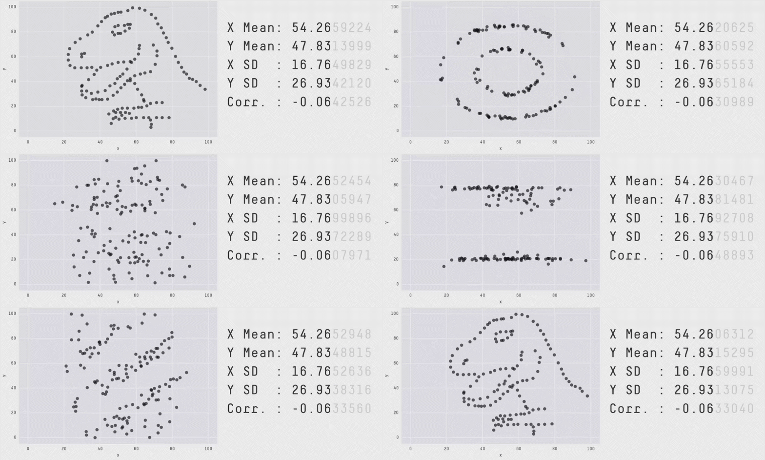
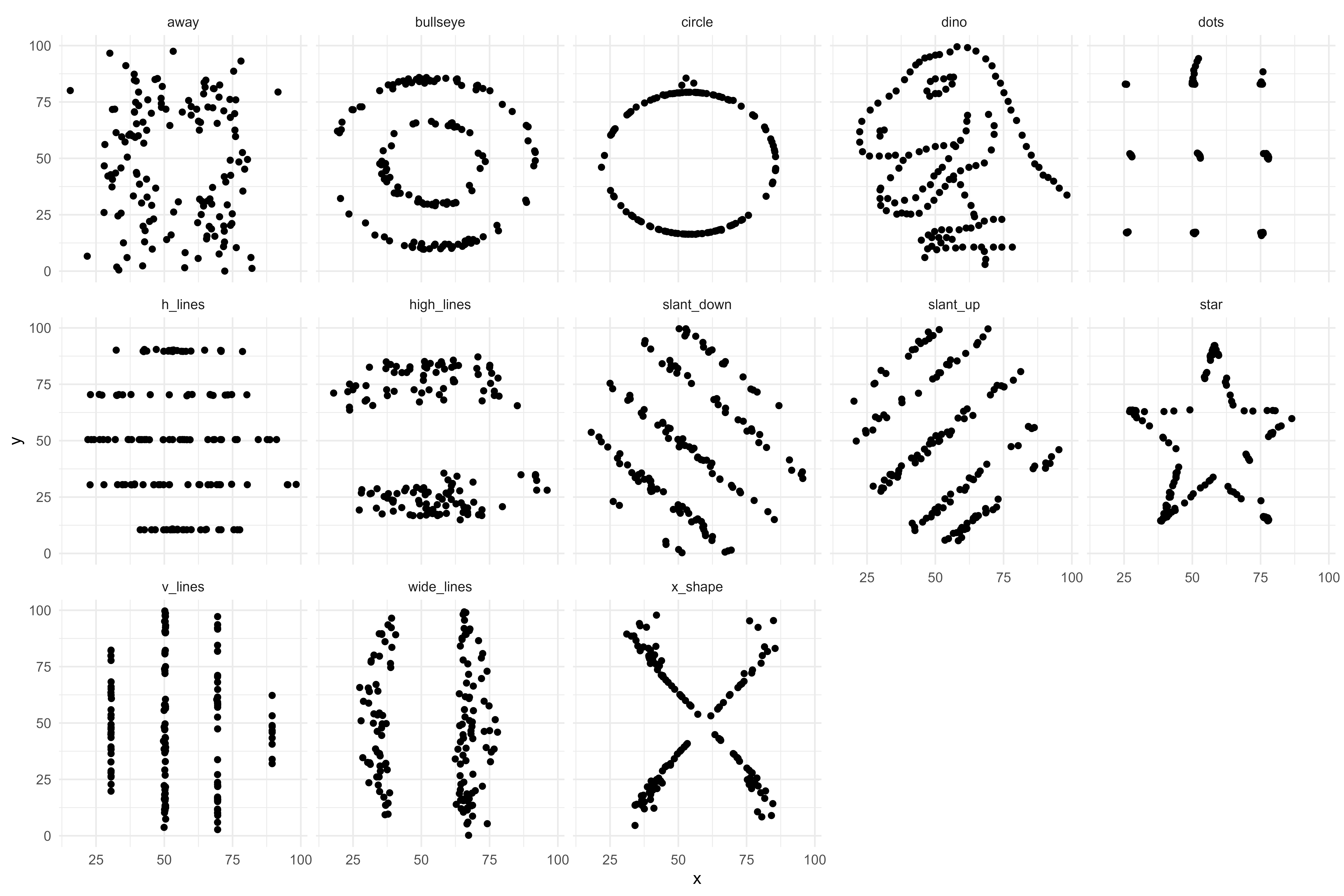
Datasaurus Dozen
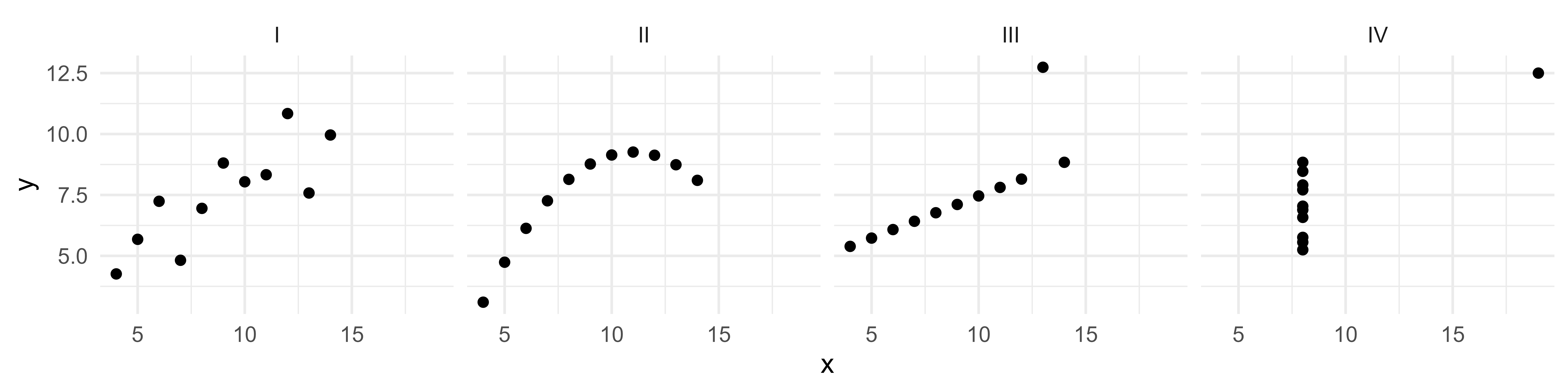
Anscombe Quartet
| dataset | n | mean_x | sd_x | mean_y | sd_y |
|---|---|---|---|---|---|
| I | 11.00 | 9.00 | 3.32 | 7.50 | 2.03 |
| II | 11.00 | 9.00 | 3.32 | 7.50 | 2.03 |
| III | 11.00 | 9.00 | 3.32 | 7.50 | 2.03 |
| IV | 11.00 | 9.00 | 3.32 | 7.50 | 2.03 |
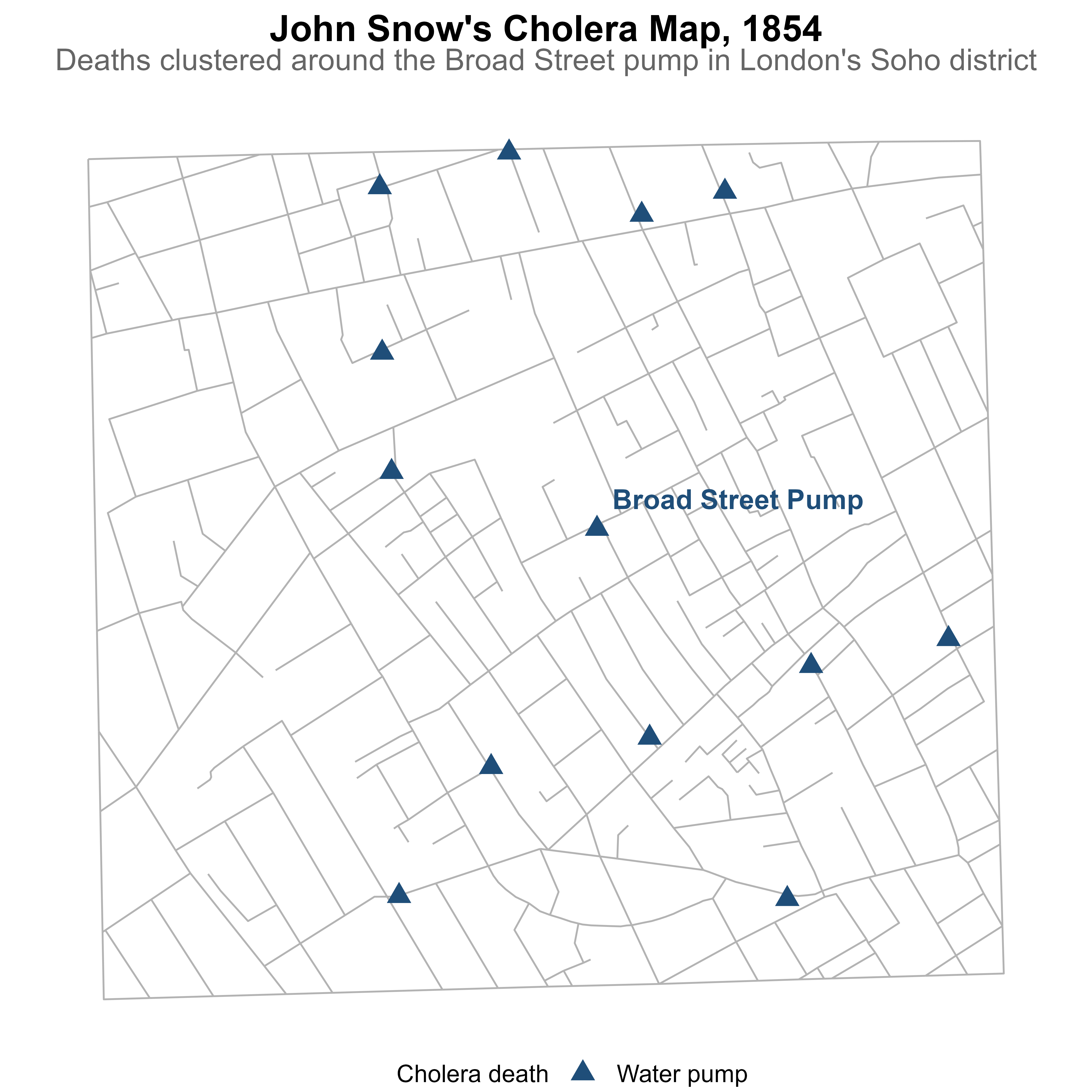
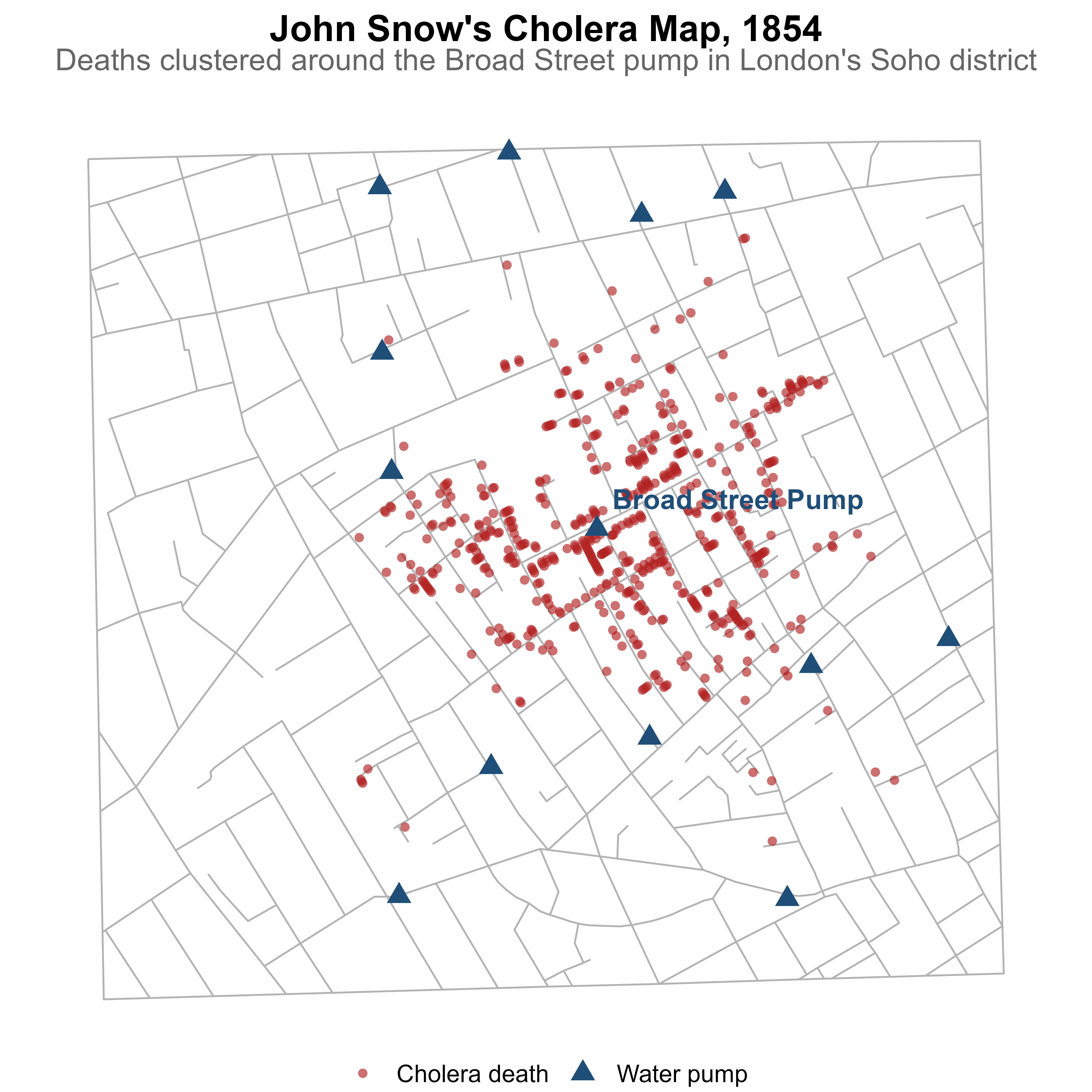
A Historical Case for Visualization
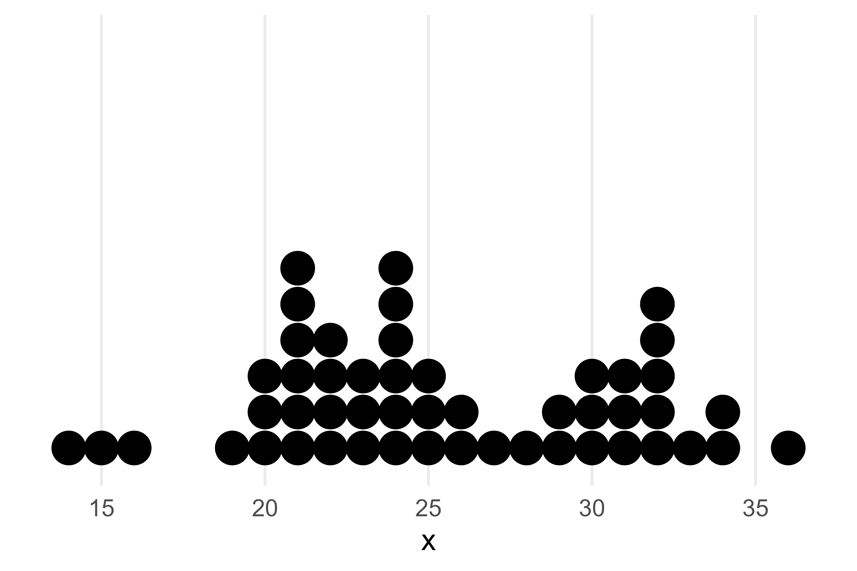
Dot plot
Useful for small to moderate sized data
Allows us to visualize the spread and distribution of a single continuous or discrete variable
- e.g. length of stay
The X axis is the variable of interest and each dot represents a single observation
Easy to identify the mode
Highlights clusters, gaps, and outliers
Intuitive and easy to understand
Histogram
Useful for all sized data (small and large)
Allows us to visualize the spread and distribution of continuous variables
Each bar represents a ‘bin’ or a defined interval of values
Although not as common, the width of the bins does NOT have to be equal!
The y axis or the height of the bar represents the count of the number of values that fall into each bin
The y axis is also commonly normalized to ‘relative’ frequencies to show the proportion of cases or density that falls into each bin.
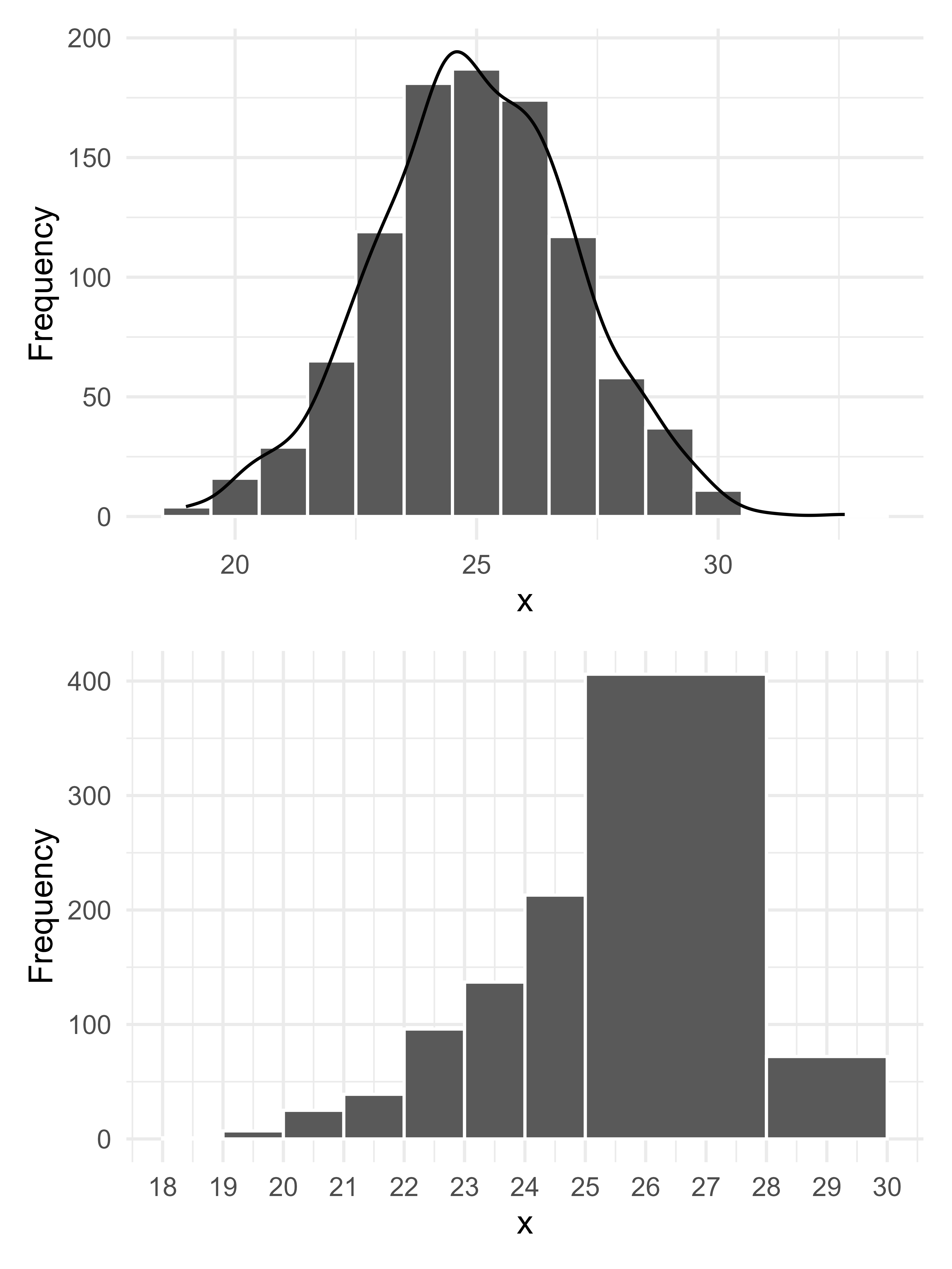
Distribution
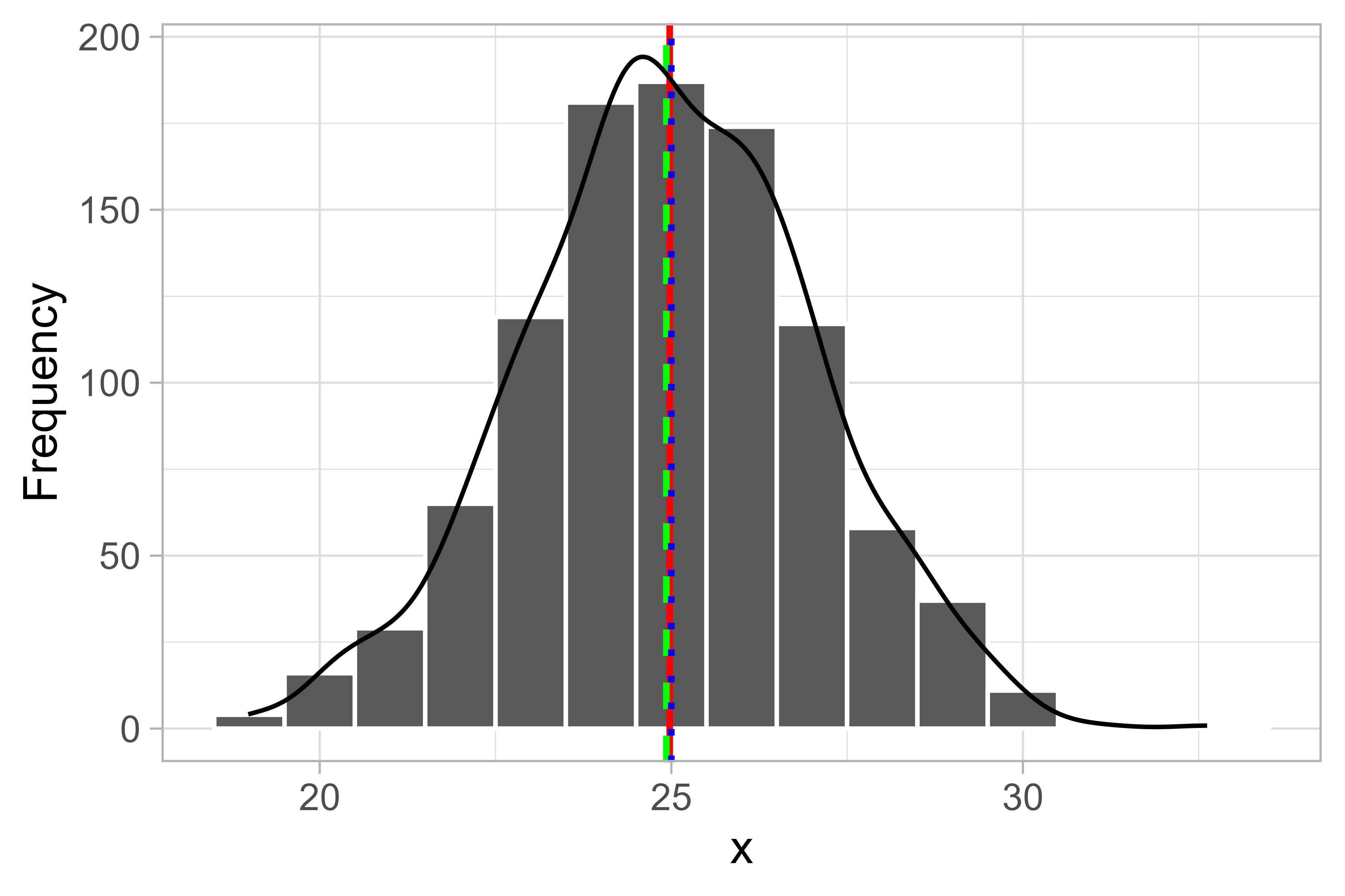
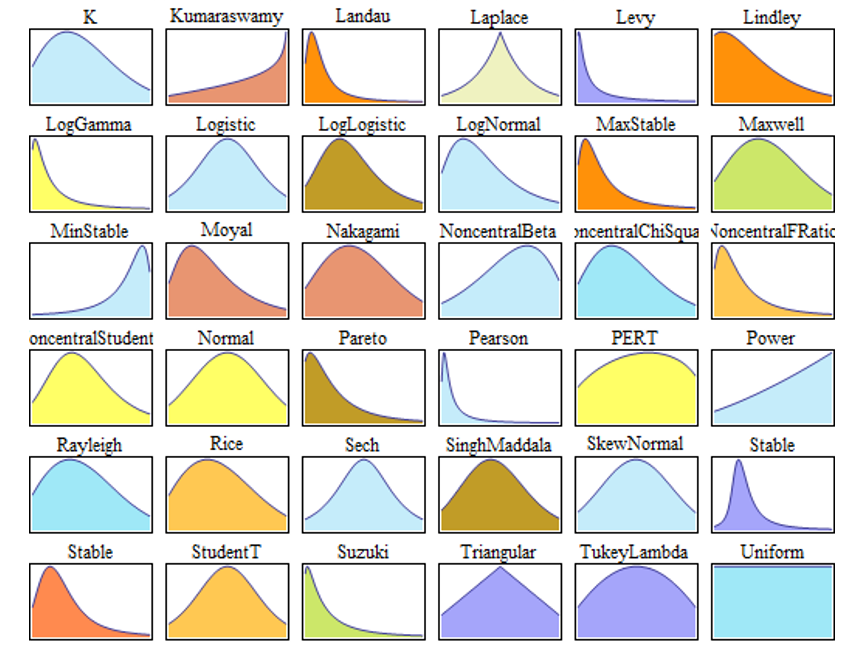
Normal Distribution
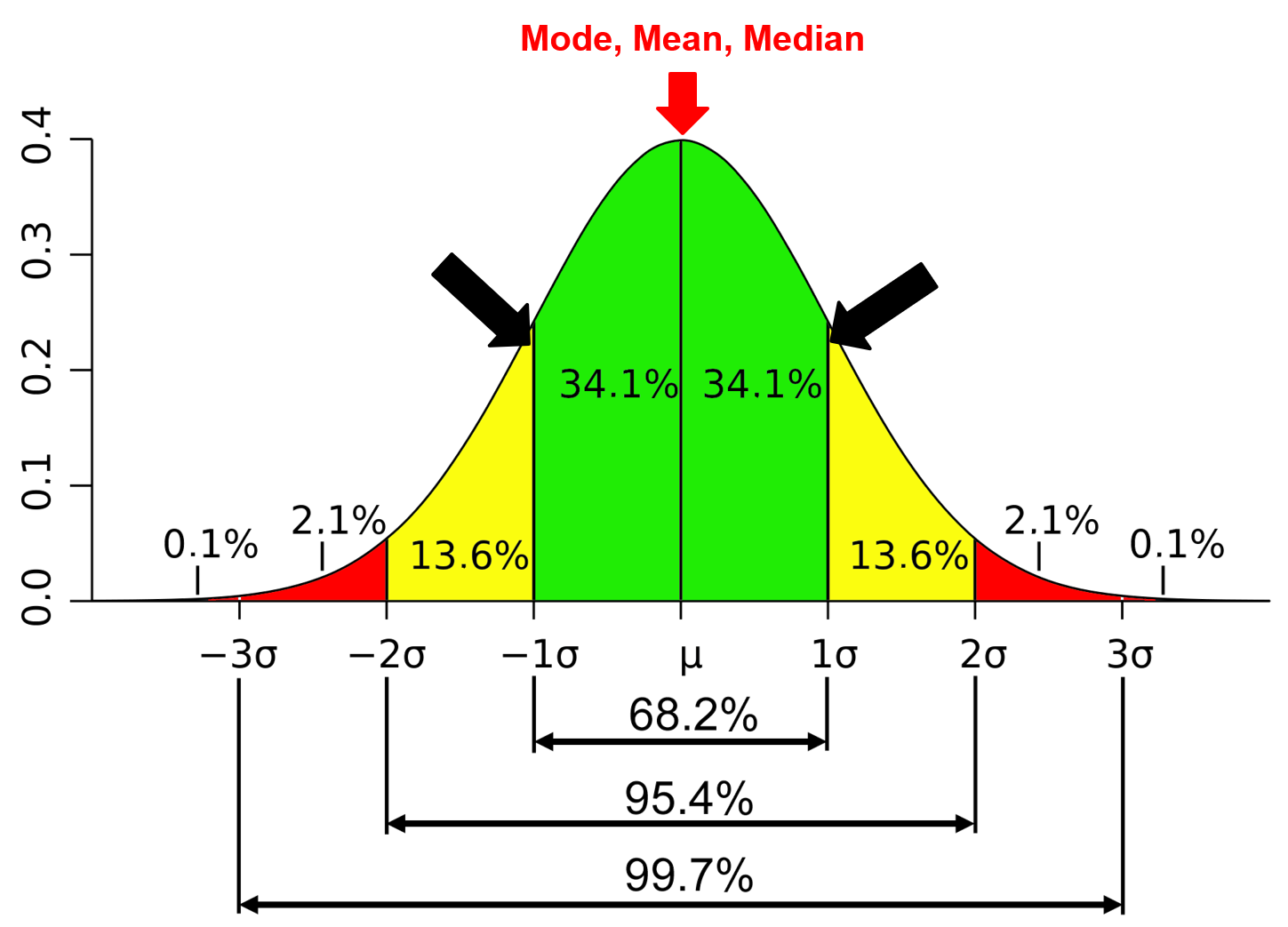
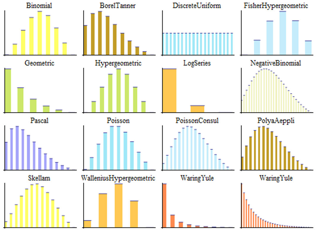
Univariate Continuous Distributions
Univariate Discrete Distributions
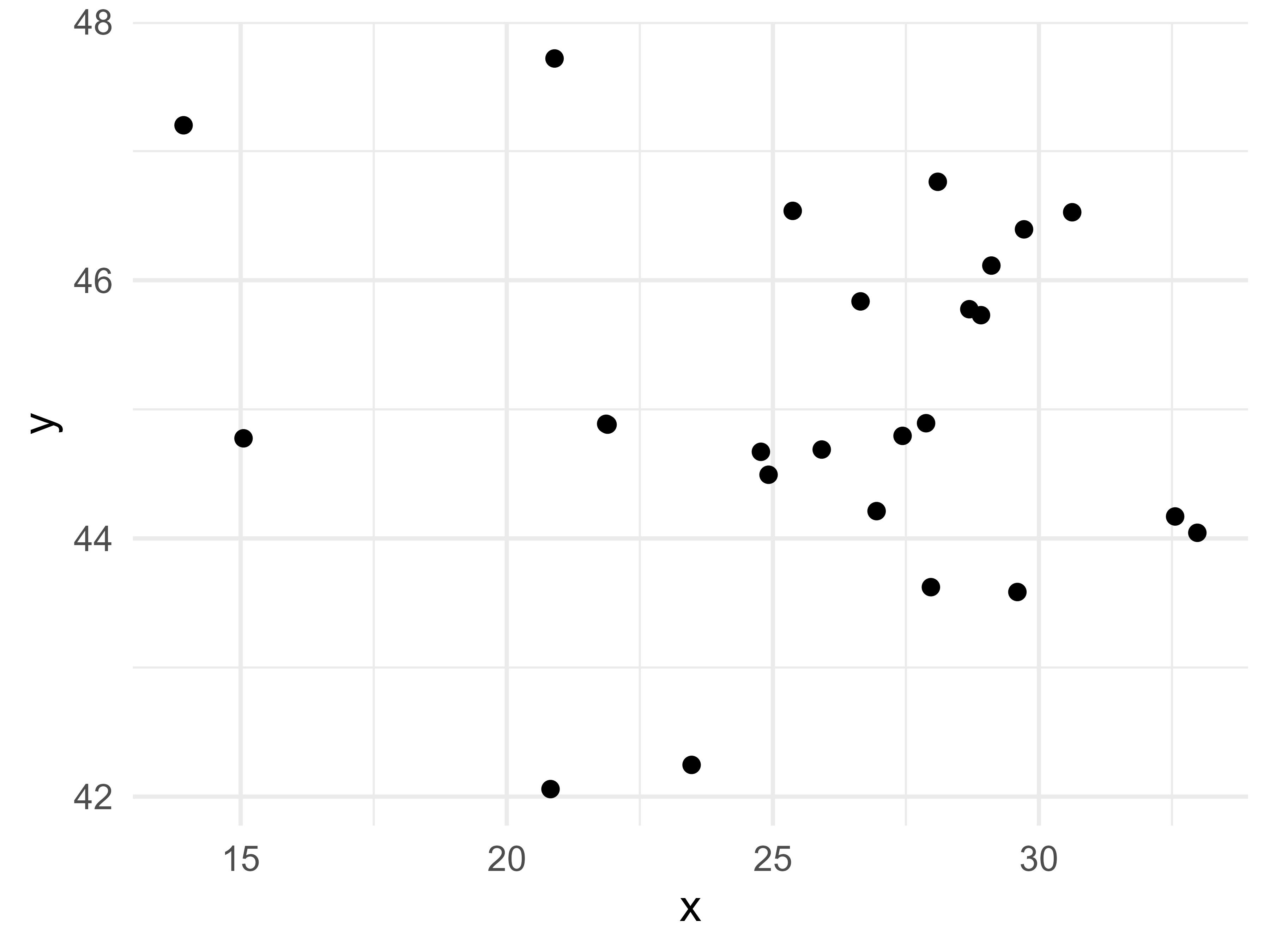
Scatter plot
Used to visualize the relationship between two continuous variables
Useful for detecting patterns that are obscured from quantitative summaries like what we observed in Anscombe’s quartet and the Datasaurus dozen.
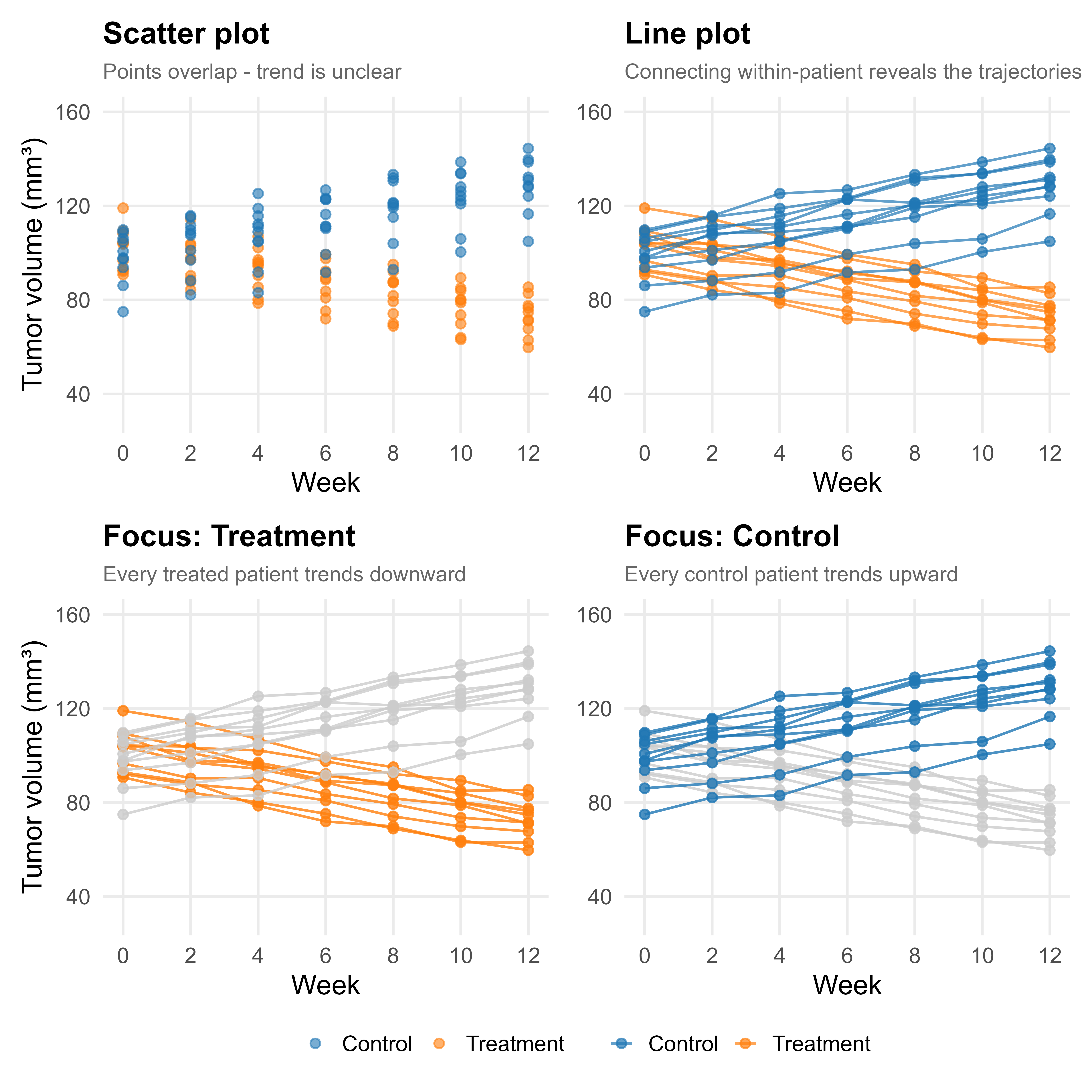
Line plot
Used to visualize a continuous variable over an ordered sequence - typically time
Points are connected in order, revealing trends and patterns of change that a scatter plot alone would obscure
Common in clinical research for tracking biomarkers, tumor burden, or patient-reported outcomes over follow-up
Multiple lines allow direct comparison between groups (e.g. treatment arms)
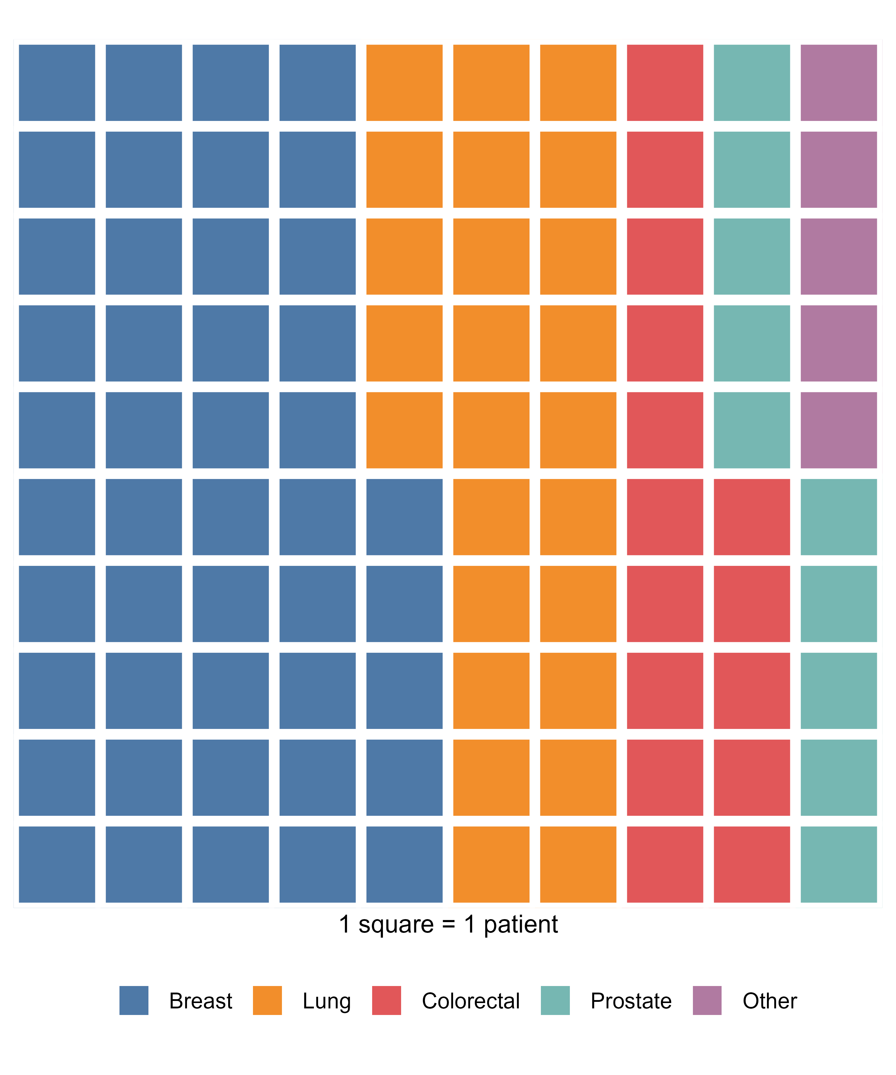
Waffle plot
- Useful for visualizing categorical data, suitable for small to moderate sized data.
- Best used when you want to emphasize the “part-to-whole” relationship in your data
- Each square represents a fixed number of observations
- Effective for communicating data to non-technical audiences
Bar plot
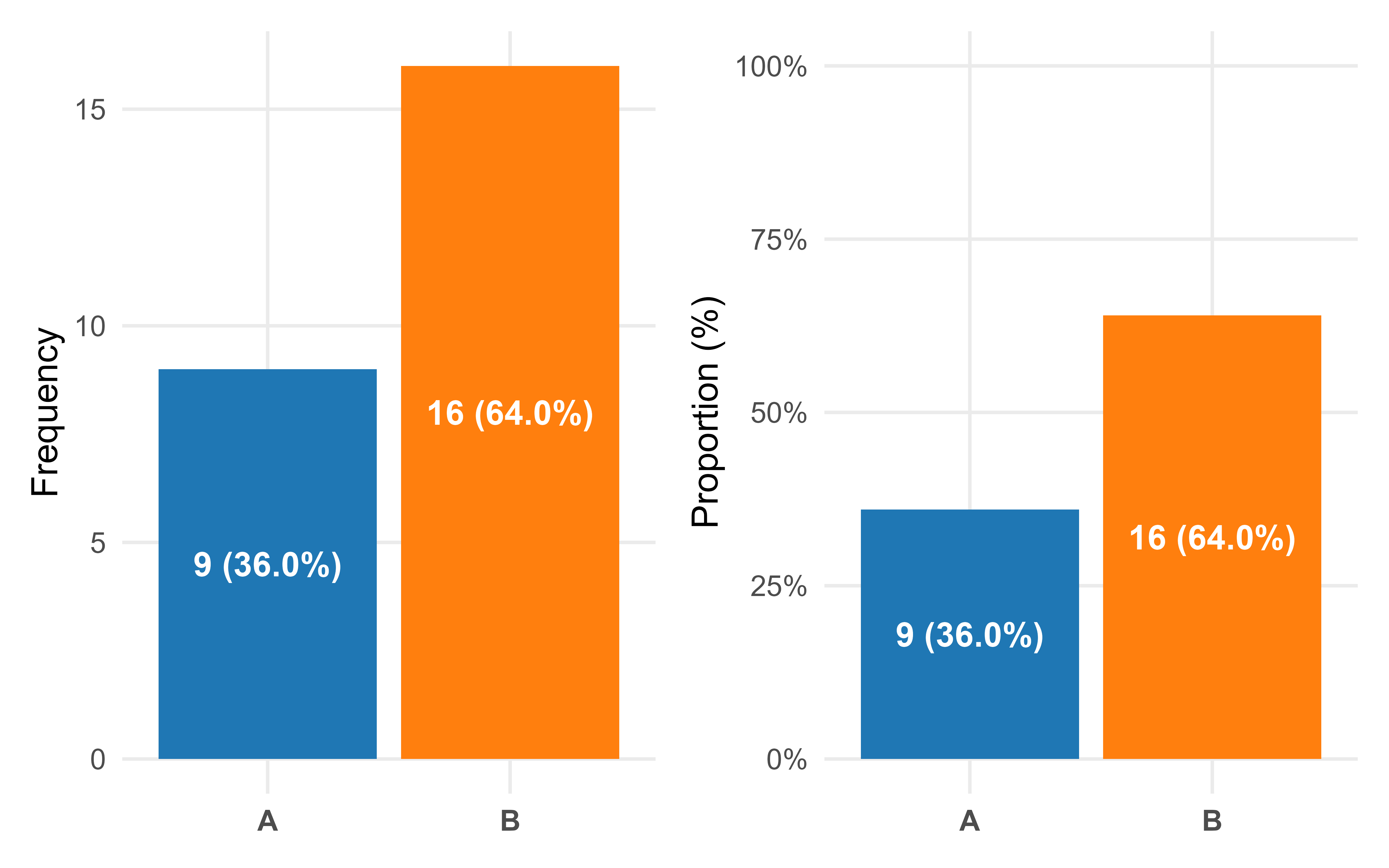
Useful for visualizing categorical data
Commonly used to present counts and proportion of each level
Allows us to quickly observe the difference in magnitude of each level based on the height of each bar
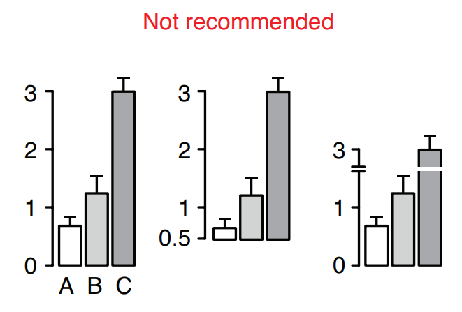
How NOT to Bar Plot
Box plot
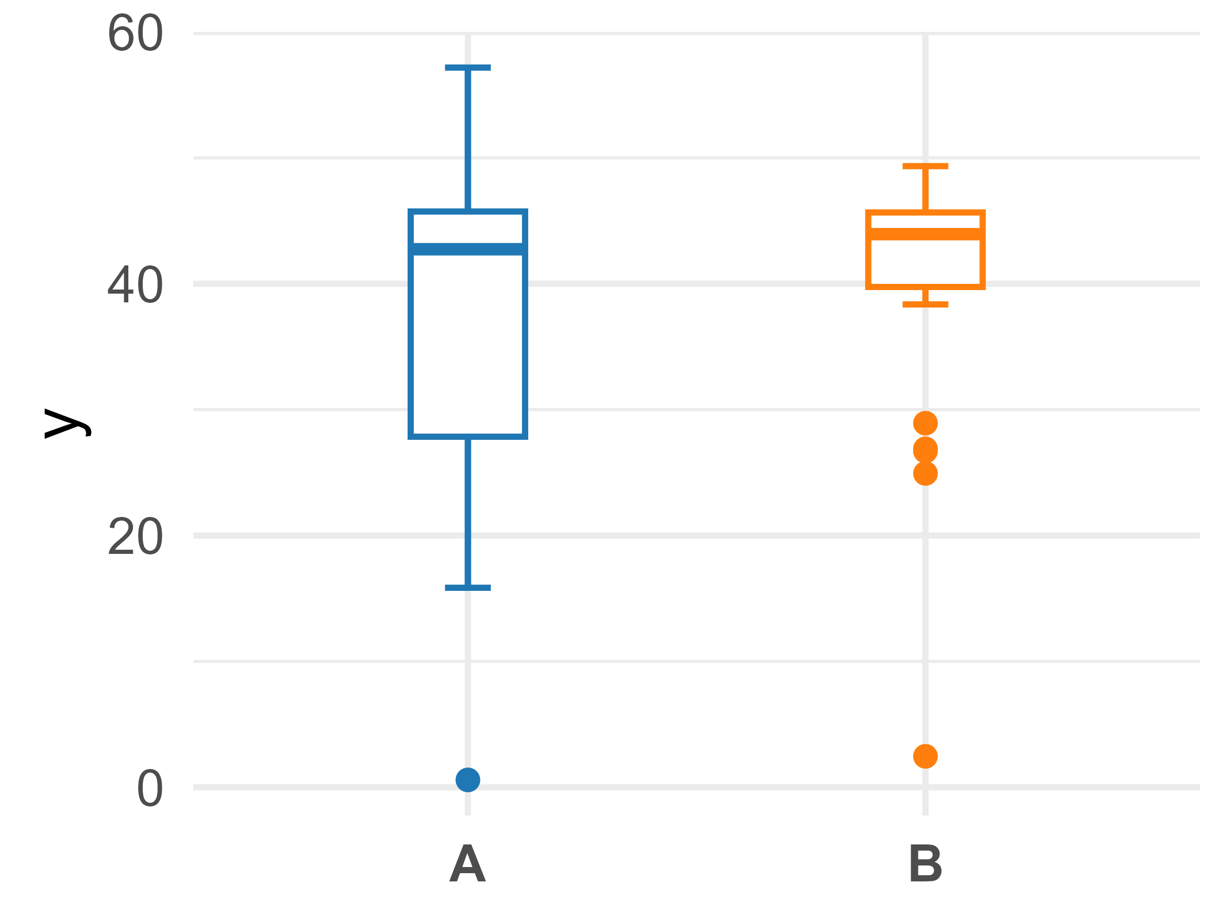
- Useful for describing continuous variables following a uni-modal distribution
- e.g. a single peak
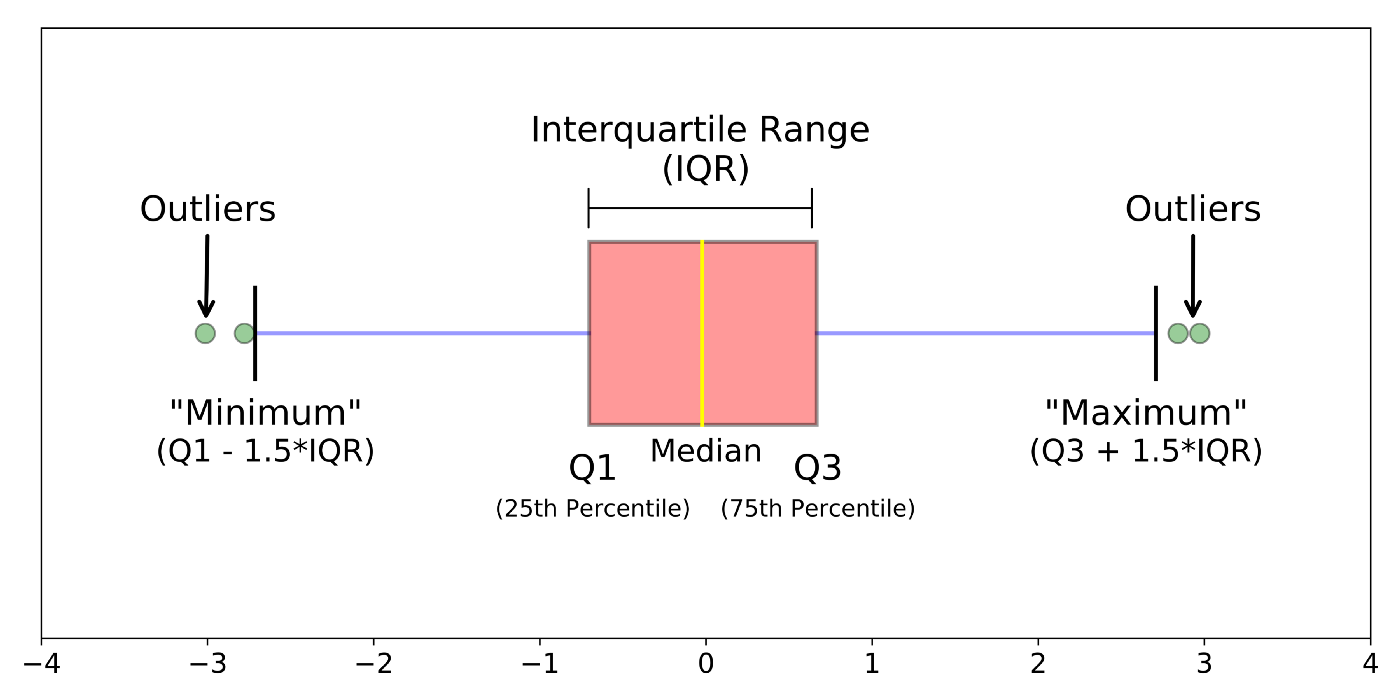
- The box is representative of common quantitative measures
- Top of box is the 75th quantile
- Middle dash inside box is the 50th quantile
- Bottom of box is the 25th quantile
- Width of the box is the interquartile range (IQR)
- The ‘whiskers’ are artificial ‘fences’ that helps identify potential outliers in the data
- Defined as Q1 - 1.5*IQR and Q3 + 1.5*IQR
Box plot
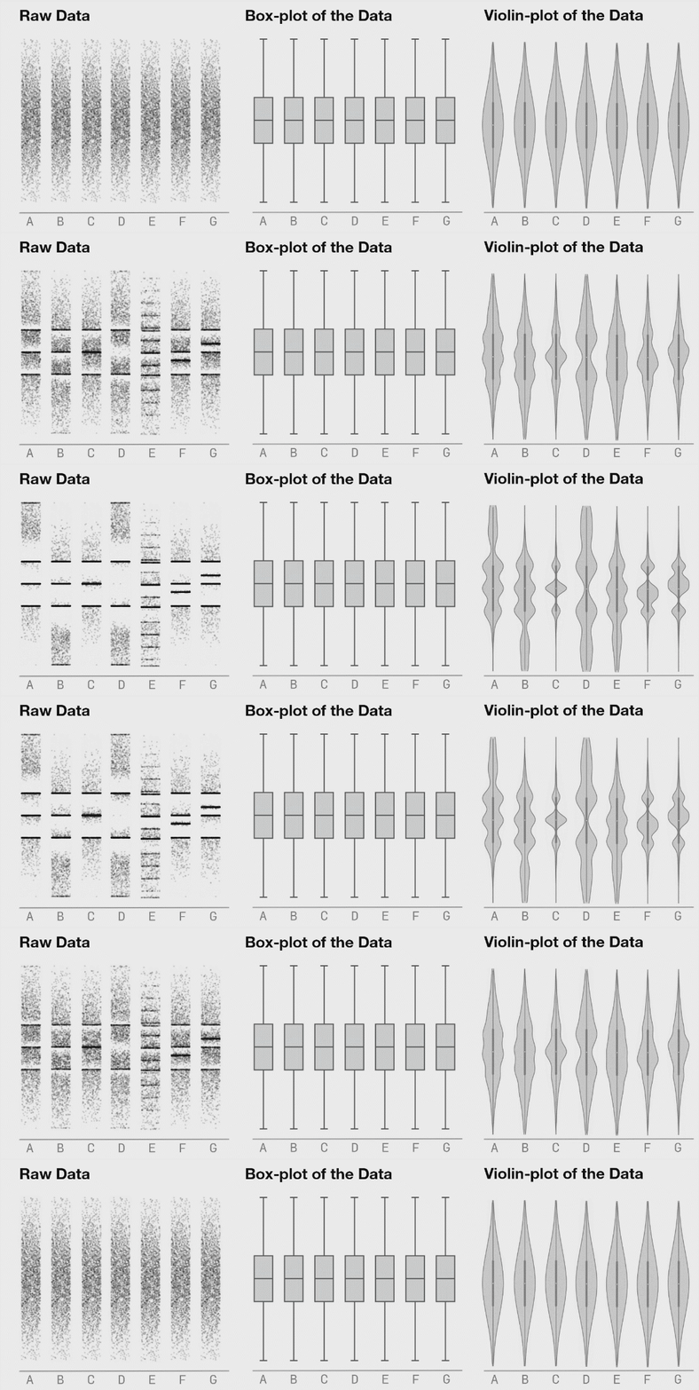
Violin plot
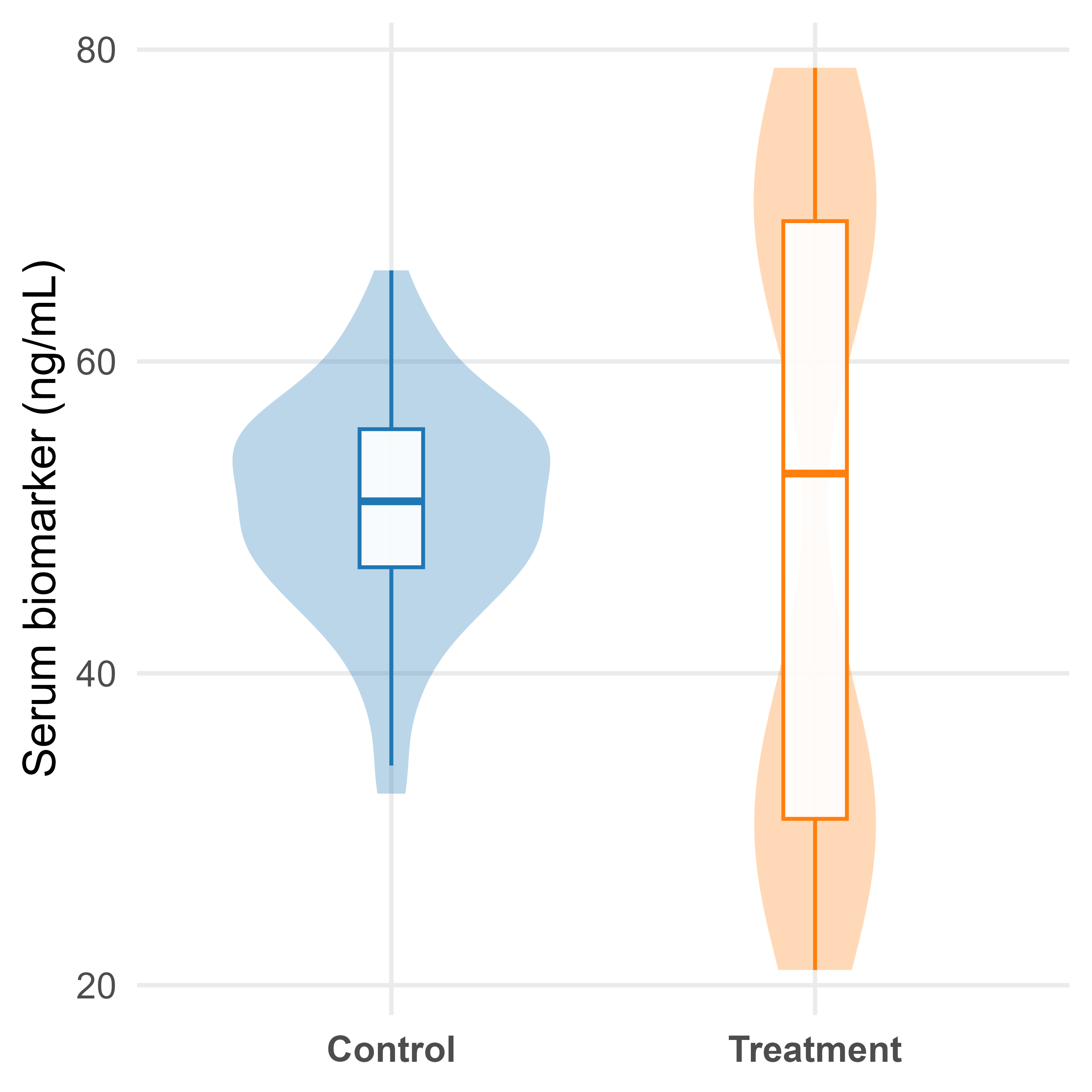
Violin plots are box plots, with an overlay of the density distribution (histogram) of the data
More informative than a simple box plot
Visualizes the full distribution of the data
Especially useful for bimodal or multimodal distribution
- e.g. distribution of data with multiple peaks
Bubble Plot
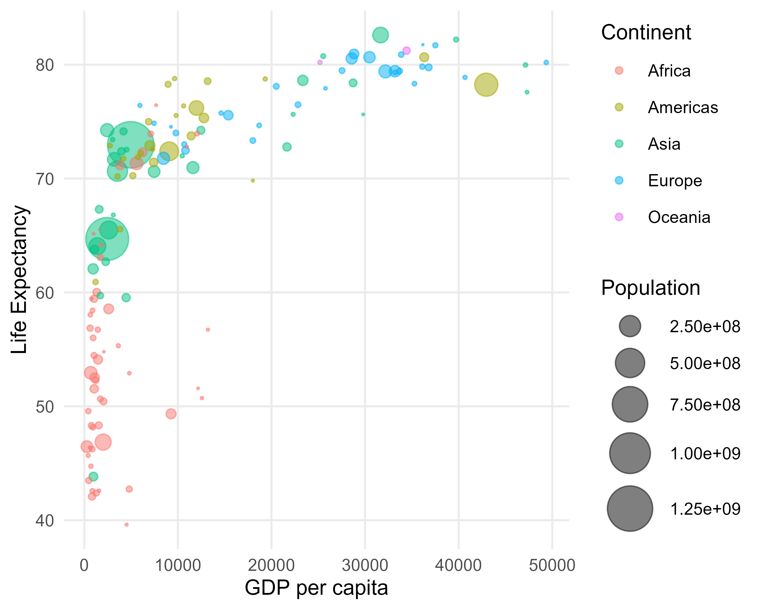
- Visualizes the relationship between two continuous variables, with a third continuous variable represented by the size of the bubbles.
- The color of the bubbles can represent a fourth categorical or continuous variable.
- Useful for identifying patterns, trends, and clusters in multivariate data.
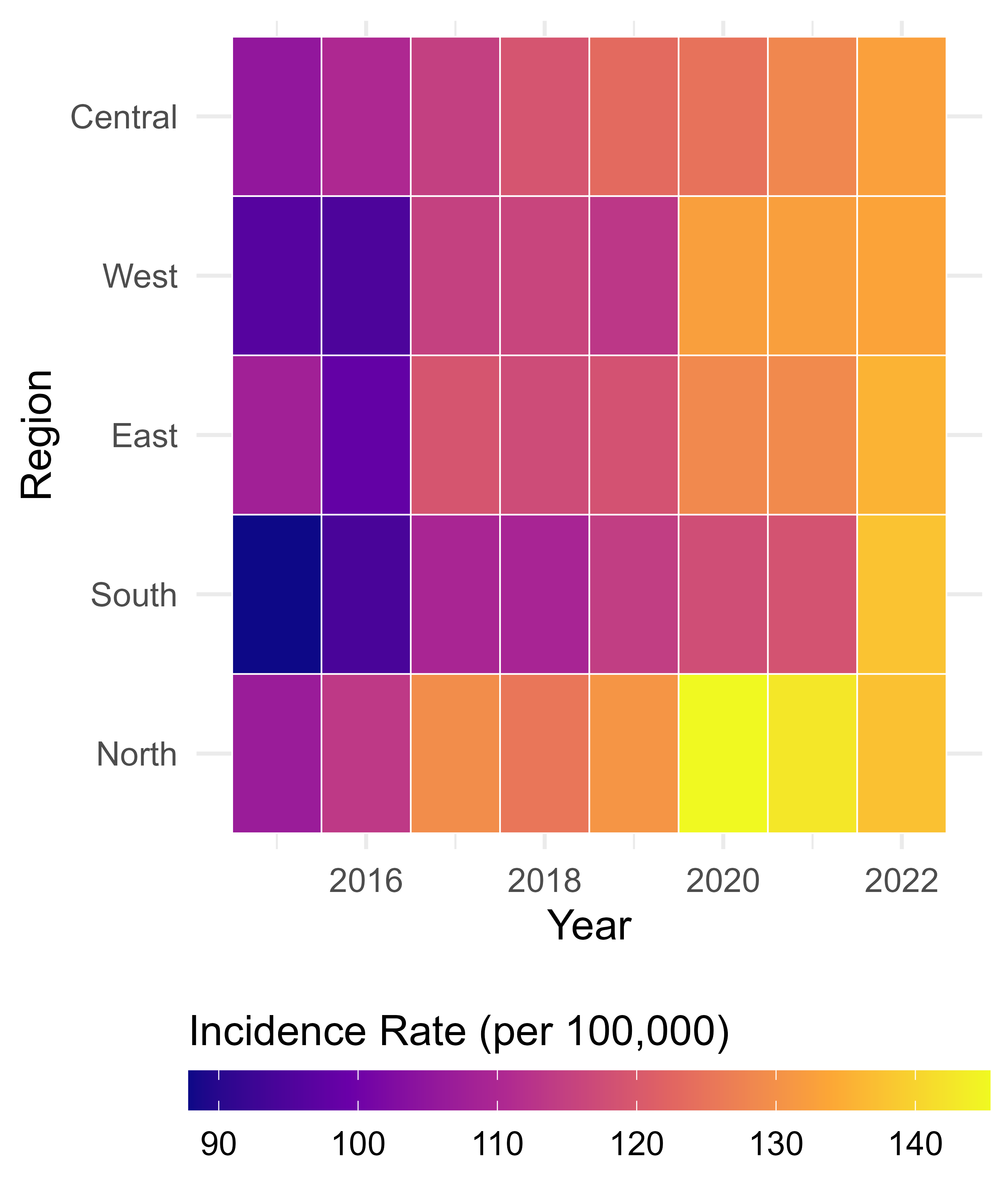
Tile Plots / Heatmaps
- Used to visualize the relationship between two categorical variables, with a continuous variable represented by color intensity.
- The color gradient can represent a summary statistic (e.g., mean, median, count) for each combination of the two categorical variables.
- Useful for identifying patterns, trends, and outliers in multivariate categorical data.