library(tidyverse)
library(tidymodels)

One of the premiere machine learning modules in python is scikit-learn and it’s going to be the first place I’m going to start in my journey of learning the python language. I am going to go through the process of building a simple logistic regression model using the tidymodels package in R, and compare it to the process of scikit-learn in python.

In this example, I will be using the palmerpenguins dataset found in the below link.

url <- 'https://gist.githubusercontent.com/slopp/ce3b90b9168f2f921784de84fa445651/raw/4ecf3041f0ed4913e7c230758733948bc561f434/penguins.csv'

The overall goal is to do a series of very standard steps in training a binary classifier (Logistic Regression).

Read in the dataset
Split the dataset into a training and testing set
Train the model on the training set
Evaluate the model on the testing set

tidymodels

Let’s start off with reading in the dataset in R

data <- read_csv(url, show_col_types = FALSE)

data

# A tibble: 344 × 9
   rowid species island    bill_length_mm bill_depth_mm flipper_length_mm
   <dbl> <chr>   <chr>              <dbl>         <dbl>             <dbl>
 1     1 Adelie  Torgersen           39.1          18.7               181
 2     2 Adelie  Torgersen           39.5          17.4               186
 3     3 Adelie  Torgersen           40.3          18                 195
 4     4 Adelie  Torgersen           NA            NA                  NA
 5     5 Adelie  Torgersen           36.7          19.3               193
 6     6 Adelie  Torgersen           39.3          20.6               190
 7     7 Adelie  Torgersen           38.9          17.8               181
 8     8 Adelie  Torgersen           39.2          19.6               195
 9     9 Adelie  Torgersen           34.1          18.1               193
10    10 Adelie  Torgersen           42            20.2               190
# ℹ 334 more rows
# ℹ 3 more variables: body_mass_g <dbl>, sex <chr>, year <dbl>

Since logistic regression is a binary classifier, we will convert the species variable into a binary outcome. The outcome we are going to train the model for is ‘Chinstrap’ vs ‘Not Chinstrap’.

data <- data |> 
  mutate(
    outcome = case_when(
      species == 'Chinstrap' ~ 1,
      .default = 0
    ),
    outcome = factor(outcome)
  )

Now that we have the outcome coded, we can split the data into a training and testing set. We will use the initial_split function from the rsample package to split the data into a 75/25 split.

set.seed(1)
split <- initial_split(data, strata = outcome)

train <- training(split)
test <- testing(split)

train

# A tibble: 258 × 10
   rowid species island    bill_length_mm bill_depth_mm flipper_length_mm
   <dbl> <chr>   <chr>              <dbl>         <dbl>             <dbl>
 1     1 Adelie  Torgersen           39.1          18.7               181
 2     2 Adelie  Torgersen           39.5          17.4               186
 3     5 Adelie  Torgersen           36.7          19.3               193
 4     9 Adelie  Torgersen           34.1          18.1               193
 5    10 Adelie  Torgersen           42            20.2               190
 6    12 Adelie  Torgersen           37.8          17.3               180
 7    13 Adelie  Torgersen           41.1          17.6               182
 8    14 Adelie  Torgersen           38.6          21.2               191
 9    15 Adelie  Torgersen           34.6          21.1               198
10    16 Adelie  Torgersen           36.6          17.8               185
# ℹ 248 more rows
# ℹ 4 more variables: body_mass_g <dbl>, sex <chr>, year <dbl>, outcome <fct>

test

# A tibble: 86 × 10
   rowid species island    bill_length_mm bill_depth_mm flipper_length_mm
   <dbl> <chr>   <chr>              <dbl>         <dbl>             <dbl>
 1     3 Adelie  Torgersen           40.3          18                 195
 2     4 Adelie  Torgersen           NA            NA                  NA
 3     6 Adelie  Torgersen           39.3          20.6               190
 4     7 Adelie  Torgersen           38.9          17.8               181
 5     8 Adelie  Torgersen           39.2          19.6               195
 6    11 Adelie  Torgersen           37.8          17.1               186
 7    18 Adelie  Torgersen           42.5          20.7               197
 8    21 Adelie  Biscoe              37.8          18.3               174
 9    35 Adelie  Dream               36.4          17                 195
10    38 Adelie  Dream               42.2          18.5               180
# ℹ 76 more rows
# ℹ 4 more variables: body_mass_g <dbl>, sex <chr>, year <dbl>, outcome <fct>

Now that we have the data split, we can pre-process the data using the recipe package. Within recipe, we will define the outcome variable outcome as well as define the predictor variables bill_length_mm, bill_depth_mm, flipper_length_mm, and body_mass_g. Since there are a number of missing data, we are going to use the step_impute_bag function to impute the missing data. We will then normalize the predictor variables using the step_normalize function.

rec <-
  recipe(outcome ~ bill_length_mm + bill_depth_mm + flipper_length_mm + body_mass_g,
         data = data) |>
  step_impute_bag(all_predictors()) |>
  step_scale(all_numeric_predictors())

rec

── Recipe ──────────────────────────────────────────────────────────────────────

── Inputs

Number of variables by role

outcome:   1
predictor: 4

── Operations

• Bagged tree imputation for: all_predictors()

• Scaling for: all_numeric_predictors()

Next we are going to define a logistic regression model specification using the logistic_reg function from the parsnip package. We will also define the engine as ‘glm’ and the mode as ‘classification’.

glm_spec <- logistic_reg() |> 
  set_engine('glm') |> 
  set_mode('classification')

glm_spec

Logistic Regression Model Specification (classification)

Computational engine: glm

Now we are going to combine the recipe and model specification into a workflow using the workflow function from the workflows package. We will then use the last_fit function to train the model in the training set, and assess the model on the testing set.

wf <- workflow(rec, glm_spec)

lf <- last_fit(wf, split)

→ A | warning: All predictors are missing; cannot impute

There were issues with some computations   A: x1

→ B | warning: glm.fit: fitted probabilities numerically 0 or 1 occurred

There were issues with some computations   A: x1
There were issues with some computations   A: x2   B: x1

lf

# Resampling results
# Manual resampling 
# A tibble: 1 × 6
  splits           id               .metrics .notes   .predictions .workflow 
  <list>           <chr>            <list>   <list>   <list>       <list>    
1 <split [258/86]> train/test split <tibble> <tibble> <tibble>     <workflow>

There were issues with some computations:

  - Warning(s) x2: All predictors are missing; cannot impute
  - Warning(s) x1: glm.fit: fitted probabilities numerically 0 or 1 occurred

Run `show_notes(.Last.tune.result)` for more information.

We can then assess the performance of the model on the test set using the conf_mat function from the yardstick package.

cm <- lf |> 
  collect_predictions() |> 
  conf_mat(truth = outcome, estimate = .pred_class)

cm

          Truth
Prediction  0  1
         0 68  2
         1  0 15

summary(cm, event_level = 'second')

# A tibble: 13 × 3
   .metric              .estimator .estimate
   <chr>                <chr>          <dbl>
 1 accuracy             binary         0.976
 2 kap                  binary         0.923
 3 sens                 binary         0.882
 4 spec                 binary         1    
 5 ppv                  binary         1    
 6 npv                  binary         0.971
 7 mcc                  binary         0.926
 8 j_index              binary         0.882
 9 bal_accuracy         binary         0.941
10 detection_prevalence binary         0.176
11 precision            binary         1    
12 recall               binary         0.882
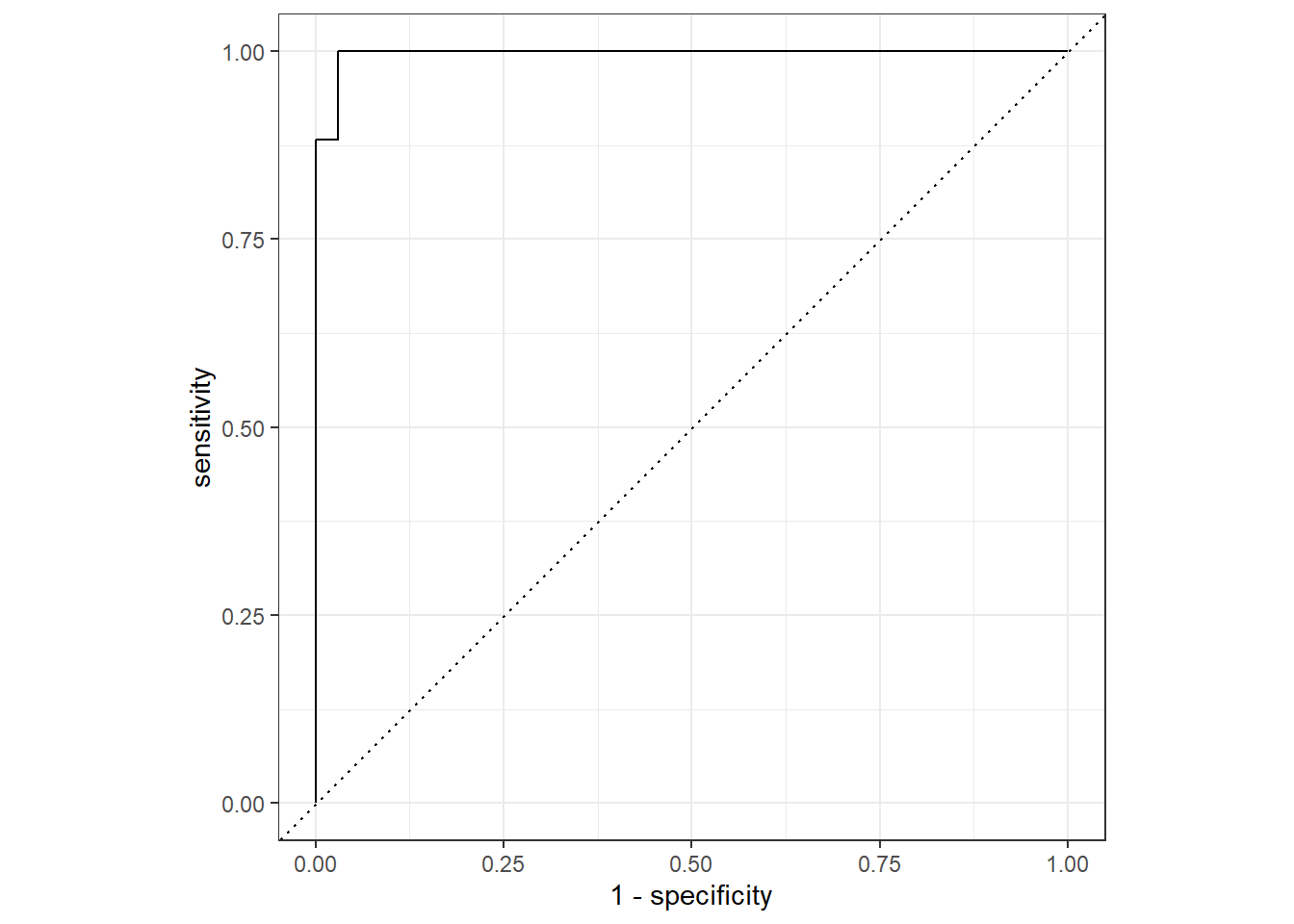
13 f_meas               binary         0.938

roc <- lf |> 
  collect_predictions() |> 
  roc_curve(truth = outcome, .pred_1, event_level = 'second') |> 
  autoplot()

roc

scikit-learn

Let’s start off with loading the pandas module and read in the dataset using the read_csv method.

import pandas as pd

url = 'https://gist.githubusercontent.com/slopp/ce3b90b9168f2f921784de84fa445651/raw/4ecf3041f0ed4913e7c230758733948bc561f434/penguins.csv'

data = pd.read_csv(url)

data

     rowid    species     island  ...  body_mass_g     sex  year
0        1     Adelie  Torgersen  ...       3750.0    male  2007
1        2     Adelie  Torgersen  ...       3800.0  female  2007
2        3     Adelie  Torgersen  ...       3250.0  female  2007
3        4     Adelie  Torgersen  ...          NaN     NaN  2007
4        5     Adelie  Torgersen  ...       3450.0  female  2007
..     ...        ...        ...  ...          ...     ...   ...
339    340  Chinstrap      Dream  ...       4000.0    male  2009
340    341  Chinstrap      Dream  ...       3400.0  female  2009
341    342  Chinstrap      Dream  ...       3775.0    male  2009
342    343  Chinstrap      Dream  ...       4100.0    male  2009
343    344  Chinstrap      Dream  ...       3775.0  female  2009

[344 rows x 9 columns]

Now that we have the data read into memory, let’s convert the species variable into a binary outcome. The most intuitive method I found to do this is to use the where method from the numpy module. This appears most similar to the mutate with the ifelse function in R.

import numpy as np

data['outcome'] = np.where(data['species'] == 'Chinstrap', 1, 0)

data

     rowid    species     island  ...     sex  year  outcome
0        1     Adelie  Torgersen  ...    male  2007        0
1        2     Adelie  Torgersen  ...  female  2007        0
2        3     Adelie  Torgersen  ...  female  2007        0
3        4     Adelie  Torgersen  ...     NaN  2007        0
4        5     Adelie  Torgersen  ...  female  2007        0
..     ...        ...        ...  ...     ...   ...      ...
339    340  Chinstrap      Dream  ...    male  2009        1
340    341  Chinstrap      Dream  ...  female  2009        1
341    342  Chinstrap      Dream  ...    male  2009        1
342    343  Chinstrap      Dream  ...    male  2009        1
343    344  Chinstrap      Dream  ...  female  2009        1

[344 rows x 10 columns]

Now that we have the outcome coded, we can split the data into a training and testing set. We will use the train_test_split method from the sklearn module to split the data into a 75/25 split. The sklearn module appears to t

from sklearn.model_selection import train_test_split

X = data.loc[:, ['bill_length_mm', 'bill_depth_mm', 'flipper_length_mm', 'body_mass_g']]
y = data.loc[:, 'outcome']

X_train, X_test, y_train, y_test = train_test_split(X, y, random_state = 1)

We will use a pipeline to pre-process the data using the KNNImputer and StandardScaler function from the sklearn module. We will then train the model using the LogisticRegression method.

from sklearn.linear_model import LogisticRegression
from sklearn.impute import KNNImputer
from sklearn.pipeline import make_pipeline
from sklearn.preprocessing import StandardScaler

pipe = make_pipeline(KNNImputer(), StandardScaler(), LogisticRegression())

pipe.fit(X_train, y_train)

Pipeline(steps=[('knnimputer', KNNImputer()),
                ('standardscaler', StandardScaler()),
                ('logisticregression', LogisticRegression())])

In a Jupyter environment, please rerun this cell to show the HTML representation or trust the notebook.
On GitHub, the HTML representation is unable to render, please try loading this page with nbviewer.org.

Now that the model is fit, let’s assess the model performance using the confusion_matrix and classification_report function from the sklearn module.

from sklearn.metrics import confusion_matrix, classification_report, roc_auc_score, RocCurveDisplay

confusion_matrix(y_test, pipe.predict(X_test))

array([[68,  0],
       [ 1, 17]], dtype=int64)

roc_auc_score(y_test, pipe.predict_proba(X_test)[:, 1])

0.9959150326797386

cr = classification_report(y_test, pipe.predict(X_test))

print(cr)

              precision    recall  f1-score   support

           0       0.99      1.00      0.99        68
           1       1.00      0.94      0.97        18

    accuracy                           0.99        86
   macro avg       0.99      0.97      0.98        86
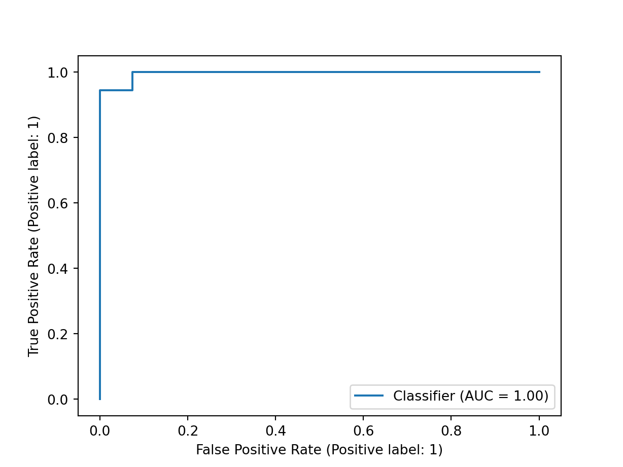
weighted avg       0.99      0.99      0.99        86

RocCurveDisplay.from_predictions(y_test, pipe.predict_proba(X_test)[:, 1])

<sklearn.metrics._plot.roc_curve.RocCurveDisplay object at 0x000001FCCBD526B0>

Reuse

CC BY 4.0

Citation

BibTeX citation:

@online{luu2024,
  author = {Luu, Michael},
  title = {Scikit-Learn {Practice} {From} the {Perspective} of an {R}
    {User}},
  date = {2024-02-02},
  langid = {en}
}

For attribution, please cite this work as:

Luu, Michael. 2024. “Scikit-Learn Practice From the Perspective of an R User.” February 2, 2024.